Deep Learning
Table of Contents
Deep Learning
You learn:
- To understand how neural networks work
- How neural networks are mathematically described
- To understand the layers of neural networks
- To program basic neural networks
- What activation functions are
- How forward- and backpropagation works
- What overfitting is and how it can be prevented
Preparation
Introduction
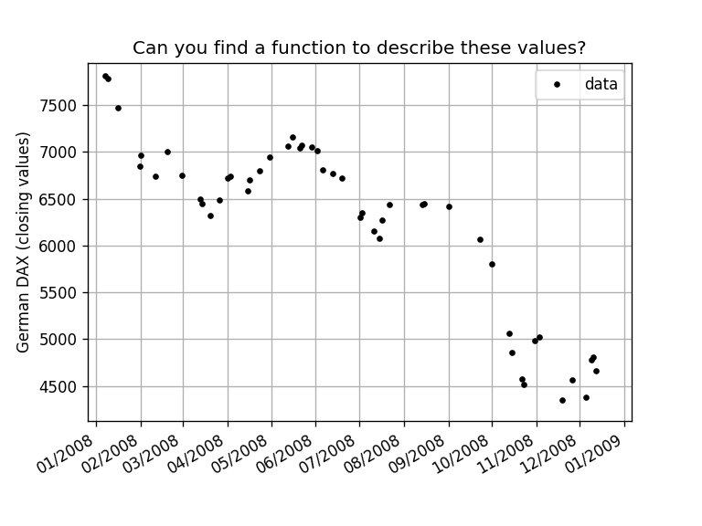
Can you find a function to describe the given data? An easy solution is to use a polynomial approximation:
$$ f(x) = \sum_{i=0}^N a_i x^i $$
By minimizing the least-squares of the polynomial and the given dataset, a solution-vector $\vec{a}$ (containing all $a_i$) can be obtained.
An optimizer to solve these problems is available, and this task can be achieved easily:
# https://numpy.org/doc/stable/reference/generated/numpy.polynomial.chebyshev.Chebyshev.fit.html
from numpy.polynomial import Chebyshev
The dataset is the German DAX stock index in 2008, the second year of the global financial crisis of 2007–2008. It contains the closing values of the stock index (i.e., its value when the market was closed after business hours). However, the dataset is incomplete; it does not contain all data but a (random) selection of 50 (tradeable) days.
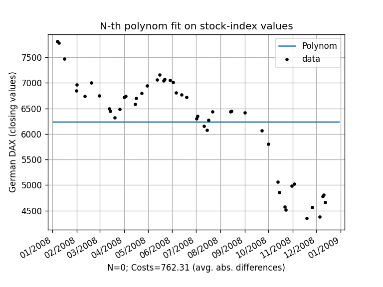
Costs for approximation of the dataset using a polynomial function (image animated)
By increasing $N$, new polynomial terms are added, and the approximation gets better as we add flexibility with every added term. A cost function is defined as the average absolute differences between the dataset and the value of the polynomial approximation at each data point. The cost is decreasing with the number of added polynomial terms. But the higher polynomials ($N > 35$) look strange. Are they representing the data or a mathematical artifact?
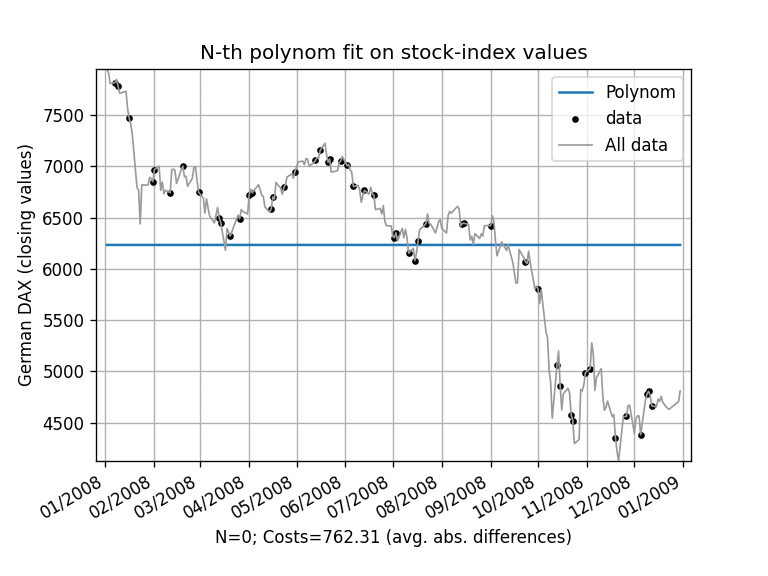
All available data with the selected dataset and the polynomial approximation (image animated)
In higher polynomials, the border regions (left and right) start to jitter, and the jittering moves inwards with higher polynomials. It's a mathematical artifact, as the values generated by high polynomials change very quickly. The borders of the dataset are (for polynomials) hard to fit. But why are the costs decreasing if the fitting is getting worse?
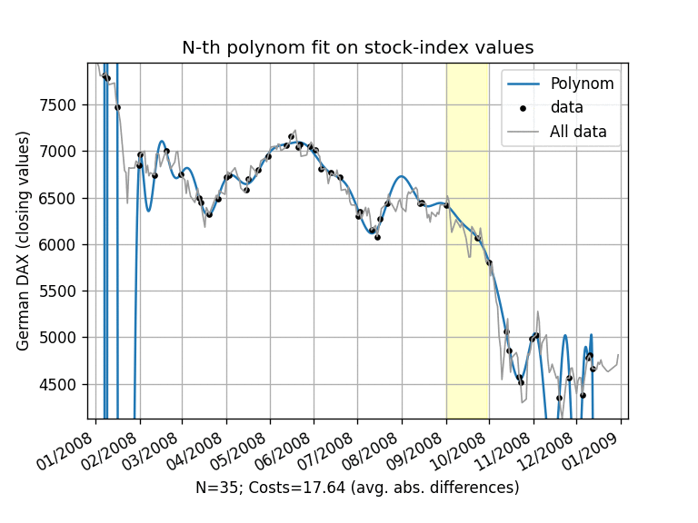
Overfitting is shown in the highlighted region (image animated)
There is an issue of overfitting. The costs decrease with more terms (degrees of freedom), but the costs are calculated on the selection and not the whole dataset. This leads to overfitting, a situation where the description of the whole data is getting worse by adding more degrees of freedom. To prevent this, two datasets, one for training and one for validation, are needed.
You've learned:
- Polynomials don't behave well (in border regions)
- More degrees of freedom results in better results (more is better)
- Overfitting is an issue (more is not always better)
- Two separate datasets: one for training and one for validation
Generalized Approach via Neurons
The polynomial fit is specific, and another algorithm is needed to approximate datasets in a more general way. One way to achieve this is the so-called neural networks (NN). NN are modeled to mimic the behavior of biological neurons. Biological neurons are activated over external signals. If the activation is sufficient enough, the neuron fires and tries to activate other neurons to which they are connected. However, an artificial NN is simply a function mapping an input vector to an output vector:
$$ f(\vec{x}) = \vec{y} $$
A Simple Neural Network
In the introductory example, the input vector has the length of one and is the time. The output vector also has the same length of one, and it represents the closing value of the stock index. The introductory problem can be written as $f(x) = y$.
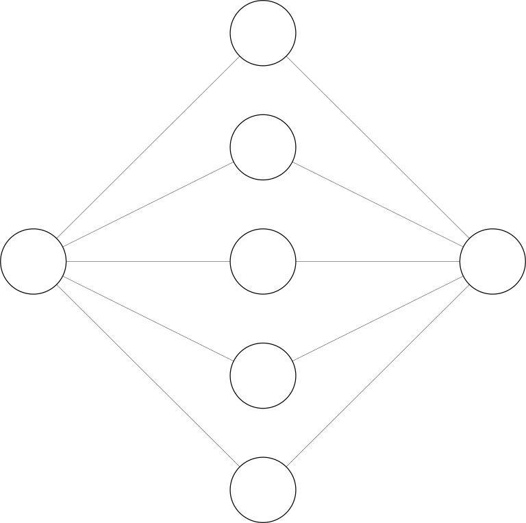
Neural network with one hidden layer
A NN is read from left to right. The left layer is the input layer $x$, and the right layer is the output layer $y$. Each node represents a neuron - a function acting on an input vector and generating a so-called activation (the function's result). Each connection drawn on the left side of a neuron represents the neuron's input vector. The NN shown in the figure above has one hidden layer with five neurons. Analog to the introductory problem, these neurons could represent one term $z_i(x) = ai x^i$ of the polynomial. The output neuron could be linear with a bias ($b$); i.e., $\sum{i=0}^N z_i(x) + b$. In this special case, the figure above would describe a 5th-grade polynomial.
It can be proven that a multi-layer representation with a single hidden layer containing a finite number of neurons can approximate any continuous function:
- Cybenko, G. Approximation by superpositions of a sigmoidal function. Math. Control Signal Systems 2, 303–314 (1989). DOI:10.1007/BF02551274
Multi-dimensional Neural Networks
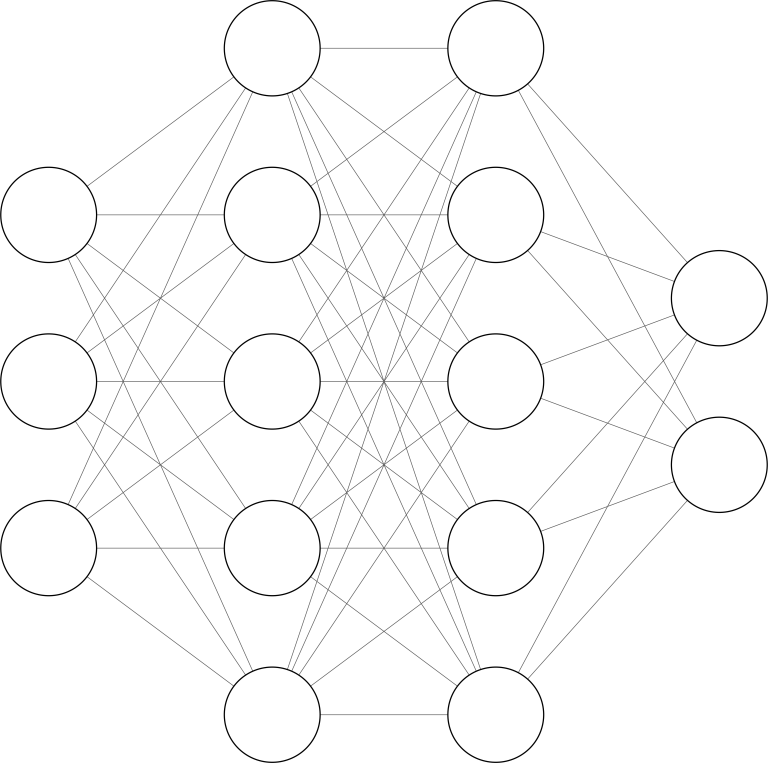
Neural network with two hidden layers
Multi-dimensional neural networks are built following a pattern. Each neuron is an activation function:
$$ \phi(z) $$
that takes the activation $z$ from its incoming connections $\vec{x}$ and applies weights $\vec{w}$ to each incoming connection and a bias $b$. The activation can be written as:
$$ z = \sum_{i=0}^N w_i \cdot x_i + b $$
Using a vector notation, the sum can be simplified to:
$$ z = \vec{w} \cdot \vec{x} + b $$
With this notation, it is also possible to calculate the activation of the whole i'th layer:
$$ \vec{a}^{(i)} = \phi(\mathbf{W} \vec{a}^{(i-1)} + \vec{b}) $$
Now all weights are aligned in a matrix, and the biases are represented by a vector. Matrix and vector multiplications are common operations, and it is easy to calculate the results of a neural network. The following example uses a sigmoid function as an activation function and calculates the results of a neural network given a bias-vector and a weights-matrix for each layer (biases and weights):
import numpy as np

def sigmoid(x):
    """
    Sigmoid activation function
    """
    return 1 / (1 + np.exp(-x))

def forward_propagation(a, weights, biases):
    """
    Calculate the results of the neural network
    """
    for b, w in zip(biases, weights):
        a = sigmoid(np.dot(w, a) + b)
    return a
Data Preprocessing
In any machine learning project in general, the data is divided into three sets:
- Training: Used to train the algorithm and construct batches
- Development: Used to finetune the algorithm and evaluate bias and variance
- Testing: Used to generalize the error/precision of the final algorithm
The sizes of each set depend on the research question, used method, and the dataset itself. Small datasets should use 60% training, 20% development, and 20% testing data. Large datasets can use 96% data for training and 2% each for development and testing.
- Tsamardinos, I., Greasidou, E. & Borboudakis, G. Bootstrapping the out-of-sample predictions for efficient and accurate cross-validation. Mach Learn 107, 1895–1922 (2018). DOI:10.1007/s10994-018-5714-4
Furthermore, it's also recommended to normalize the dataset. Having a large range (i.e., 4000 in the example from the introduction) leads to a large search space and decreases the performance.
Deep Learning as a Supervised Task
Most deep learning problems tend to predict an output using a set of variables. One application is Image-Classification, where a dataset consists of labeled images; for example, the image of a hand-written number with the label which number is shown. If the images are gray-scale and scaled to the same size, each image can be written as a vector, where each element corresponds to the brightness (0-100%) of a pixel. The output of the NN contains ten elements, each representing one label.
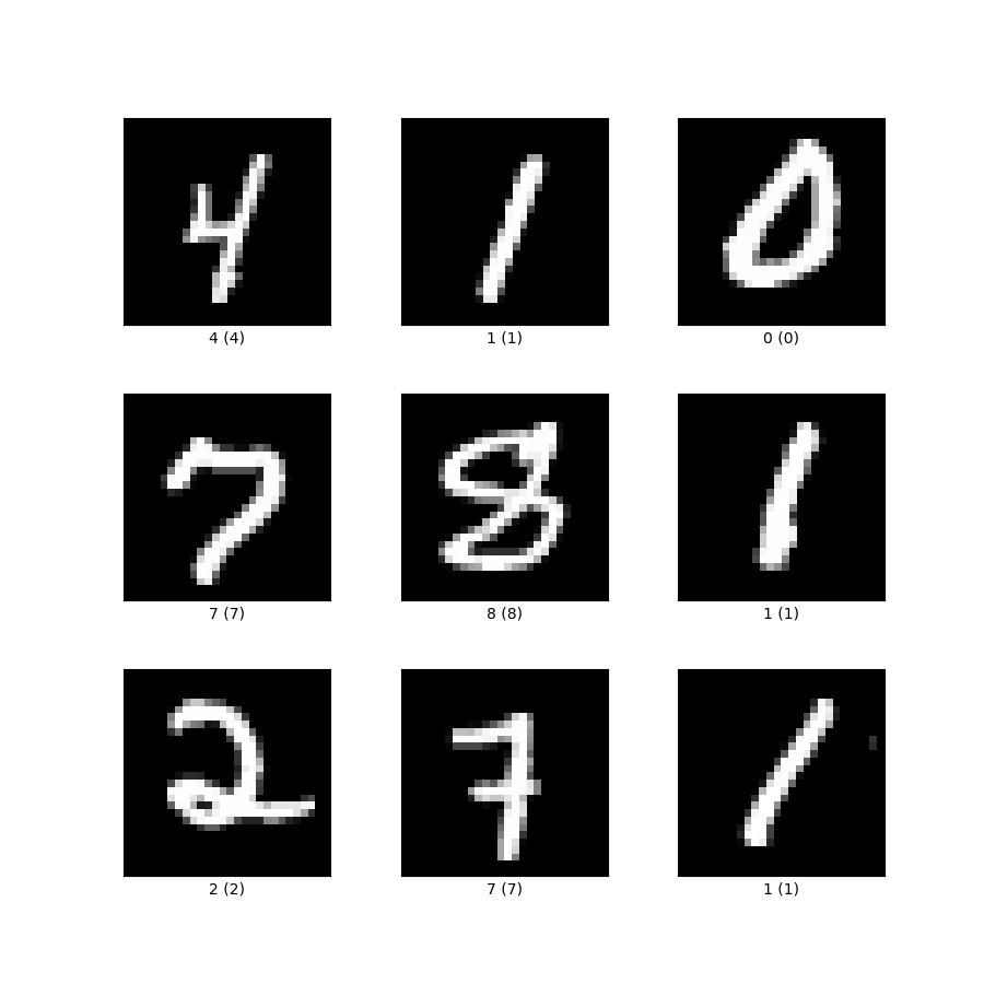
MNIST dataset; image from TensorFlow Datasets
Forward Propagation
The calculation of the results is straightforward and was explained previously. But the previous solution can be refined further to process batches of $\vec{x}$. The following indices are used:
- $k$ for the position of the data in the dataset (or selection/batch)
- $i$ for the position of the corresponding neuron in layer L
- $j$ for the position of the corresponding neuron in layer (L-1)
- The layer of a variable is given via a superscript in brackets $v^{(L)}$ or $v^{(0)}$
The matrix elements of the $L$'th layer activation function are written as:
$$ a{ik}^{(L)} = \phi^{(L)}(z{ik}^{(L)}). $$
And the activation matrix elements are calculated by:
$$ z_{ik}^{(L)} = \sumj^{(L)} w{ij}^{(L)} \cdot a{ik}^{(L-1)} + b{i}^{(L)}. $$
Please note that the index on $a$ should be $j$, but is written as $i$, because $a$ is taken from the previous layer. $b{i}^{(L)}$ is a vector; when writing $z{ik}^{(L)}$ as a matrix equation, the addition of vectors and matrices is an invalid mathematical operation. This can be solved either programmatically or by creating an $i \times k$ matrix (on the fly), which contains the same values in every row. For the first layer, an $x{ik}$ matrix can be used to propagate a list of $k$ inputs. By keeping the indices consistent, this representation can be used to derive matrix operations for efficient forward propagation. This adds additional rules, as matrices usually don't commute and need to be transposed to change the order of indices. $z{ik}^{(L)}$ can be calculated by matrix multiplication and addition if it is used as written.
Network Initialization
The biases and weights of a neural network are generated when the network is initialized. A Zero initialization sets all parameters to zero. The forward propagation equations yield hidden units that will be symmetric, which penalizes the learning phase. In random initialization, all weights and biases are set to random values. It's commonly used, but if the noise is too large, some activation functions might get saturated, which might affect the computation of the gradient.
- See Glorot et al. Understanding the difficulty of training deep feedforward neural networks for a more detailed view on the difficulty of training deep feedforward neural networks.
A saturated NN is one where most of the hidden nodes have values close to their mathematical limits. Saturation needs to be prevented.
Cost Function
A cost function is used to determine how good (or better: how bad) the NN model is. An arbitrary function can be selected, but the most common is the implementation of square-root differences between the dataset and the output layer of the neural network. The costs are calculated for every output neuron and averaged over the batch size.
$$ C = \frac{1}{N} \sum{k=0}^N \sum{i} \frac{1}{2} (a{ik}^{(L)} - y{ik}^{(L)})^2 $$
Gradient Descent
With the initial guess, the cost function can be improved. It is infeasible to guess weights and biases to improve the costs because the cost function is high-dimensional as it depends on all weights and all biases of all layers. A method called "gradient descent" is used to optimize all weights and biases on all layers at the same time. In gradient descent, the derivative of a function is used to calculate the "down-hill" direction and step length. After the gradient is calculated, all variables are changed according to direction and slope. This procedure is repeated until an abort criterion is reached. Additionally, a learning rate (number) is specified to make the step-lengths configurable. Low learning rates increase the stability of the gradient-descent algorithms but also increase the time to reach a minimum. The gradient is defined by:
$$ -\nabla C = \left[ \frac{\partial{C}}{\partial{w{ij}^{(1)}}}, \frac{\partial{C}}{\partial{b{i}^{(1)}}}, \frac{\partial{C}}{\partial{w{ij}^{(2)}}}, \frac{\partial{C}}{\partial{b{i}^{(2)}}}, \dotsb , \frac{\partial{C}}{\partial{w{ij}^{(L)}}}, \frac{\partial{C}}{\partial{b{i}^{(L)}}}, \right] $$
Backpropagation
In backpropagation, the derivative of the cost function is calculated using the layers in order from last to first. The individual partial equations of $\nabla C$ are calculated by applying the product rule of derivatives.
$$ \frac{\partial{C}}{\partial{b_{i}^{(L)}}} &= \frac{1}{N} \sumk^N \frac{\partial{C}}{\partial{a{ik}^{(L)}}} \cdot \frac{\partial{a{ik}^{(L)}}}{\partial{z{ik}^{(L)}}} \cdot \frac{\partial{z{ik}^{(L)}}}{\partial{b{i}^{(L)}}} \ &= \frac{1}{N} \sumk^N (a{ik}^{(L)} - y{ik}) \cdot \frac{\partial{a{ik}^{(L)}}}{\partial{z_{ik}^{(L)}}} \cdot 1 \ &= \frac{1}{N} \sumk^N d{ik}^{(L)} $$
The gradient of $b{i}^{(L)}$ is used to define $d{ik}^{(L)}$; a new variable storing intermediate results.
$$ \frac{\partial{C}}{\partial{w_{ij}^{(L)}}} &= \frac{1}{N} \sumk^N \frac{\partial{C}}{\partial{a{ik}^{(L)}}} \cdot \frac{\partial{a{ik}^{(L)}}}{\partial{z{ik}^{(L)}}} \cdot \frac{\partial{z{ik}^{(L)}}}{\partial{w{ij}^{(L)}}} \ &= \frac{1}{N} \sumk^N (a{ik}^{(L)} - y{ik}) \cdot \frac{\partial{a{ik}^{(L)}}}{\partial{z{ik}^{(L)}}} \cdot a{ik}^{(L-1)} \ &= \frac{1}{N} \sumk^N d{ik}^{(L)} \cdot a_{ik}^{(L-1)} $$
The gradient of $w{ij}^{(L)}$ depends on $d{ik}^{(L)}$ and the activations $a_{ik}^{(L-1)}$ of the previous layer. Both weights and biases matrices are calculated using the intermediate results of the forward propagation.
$$ \frac{\partial{C}}{\partial{b_{i}^{(L-1)}}} &= \frac{1}{N} \sumk^N \frac{\partial{C}}{\partial{a{ik}^{(L)}}} \cdot \frac{\partial{a{ik}^{(L)}}}{\partial{z{ik}^{(L)}}} \cdot \frac{\partial{z{ik}^{(L)}}}{\partial{a{ik}^{(L-1)}}} \cdot \frac{\partial{a{ik}^{(L-1)}}}{\partial{z{ik}^{(L-1)}}} \cdot \frac{\partial{z{ik}^{(L-1)}}}{\partial{b{i}^{(L-1)}}} \ &= \frac{1}{N} \sumk^N d{ik}^{(L)} \cdot \frac{\partial{z{ik}^{(L)}}}{\partial{a{ik}^{(L-1)}}} \cdot \frac{\partial{a{ik}^{(L-1)}}}{\partial{z{ik}^{(L-1)}}} \cdot \frac{\partial{z{ik}^{(L-1)}}}{\partial{b{i}^{(L-1)}}} \ &= \frac{1}{N} \sumk^N d{ik}^{(L)} \cdot w{ij}^{(L)} \cdot \frac{\partial{a{ik}^{(L-1)}}}{\partial{z_{ik}^{(L-1)}}} \cdot 1 \ &= \frac{1}{N} \sumk^N d{ik}^{(L-1)} $$
$$ \frac{\partial{C}}{\partial{w_{ij}^{(L-1)}}} &= \frac{1}{N} \sumk^N \frac{\partial{C}}{\partial{a{ik}^{(L)}}} \cdot \frac{\partial{a{ik}^{(L)}}}{\partial{z{ik}^{(L)}}} \cdot \frac{\partial{z{ik}^{(L)}}}{\partial{a{ik}^{(L-1)}}} \cdot \frac{\partial{a{ik}^{(L-1)}}}{\partial{z{ik}^{(L-1)}}} \cdot \frac{\partial{z{ik}^{(L-1)}}}{\partial{w{ij}^{(L-1)}}} \ &= \frac{1}{N} \sumk^N d{ik}^{(L-1)} \cdot a_{ik}^{(L-2)} $$
The gradients of the weights and biases of the penultimate layer are calculated using the intermediate results and weights of the last layer as well as the activations of the previous layer. Both formulas can be used to generalize the calculations of previous layers. The equations are repeated until the input layer $x{ik} = a{ik}^{(0)}$ is reached.
Calculate $\partial{C} / \partial{w_{ij}^{(L-1)}}$ using the matrices $\mathbf{D}^{(L-1)}$ and $\mathbf{A}^{(L-2)}$.
Training the Network
- Create batches from the training data
- Do forward propagation
- Calculate $-\nabla C$ using backpropagation
- Propagate the weights and biases using gradient descent
- Repeat
Activation Functions
An activation function is a transfer function that selects the data propagated in the neural network. Activation functions are modeled to mimic the excitement of neurons that fire and activate following neurons if a threshold is reached.
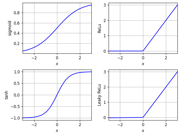
Common activation functions are:
- Sigmoid
- Hyperbolic tangent (htan)
- Rectified linear unit (ReLU) ($x$ for $x > 0$ else $0$)
Their computational performances are "ReLU" > "Tanh" > "Sigmoid", while their biological analogy is "ReLU" > "Sigmoid" > "Tanh". As Sigmoid activations are not point-symmetric, they yield poor learning dynamics when initialized from small random weights. This might lead to an initial saturation of the top hidden layer. ReLUs benefit from both linearity and nonlinearity; however, ReLUs have the problem that they might "die" in optimization because all possible inputs result in no activation. A solution to this problem is the leaky ReLu function, which has the value of $0.01 \cdot x$ for $x < 0$.
- See Glorot et al. Understanding the difficulty of training deep feedforward neural networks for a more detailed view on the difficulty of training deep feedforward neural networks.
- See Glorot et al. Deep Sparse Rectifier Neural Networks for Image Classification for a more detailed view on modeling biological neurons.
Show that $\frac{\partial}{\partial x} \tanh(x) = 1 - \tanh(x)^2$. Use $\tanh(x) = (e^{x} - e^{-x}) / (e^{x} + e^{-x})$.
Calculate $\frac{\partial}{\partial x} \sigma(x)$ with $\sigma(x) = 1 / (1 + e^(-x))$. Simplify your result until you reach a function that only depends on $\sigma(x)$.
Result => $d\sigma/dx = \sigma (1 - \sigma)$
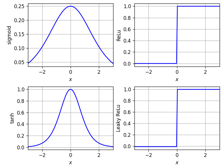
Derivatives of common activation functions
Results and Discussion
The described algorithms were implemented in Python and applied to the introductory problem. The sources and data are available:
- dax.csv: The data used to train the network
- neuralnetwork.txt: Implementation of a neural network with only numpy as dependency
- create_images.txt: Script used to create the images used in this course
You can find answers to some of this course's tasks in the implemented neural network
A 3-layer Network was built with one input, one output, and x hidden nodes in the corresponding layers ([1, x, 1]-NN). Sigmoid was used as an activation function for the second layer (according to Cybenko et al.) and a linear activation function ($f(x)=x$) for the last layer.
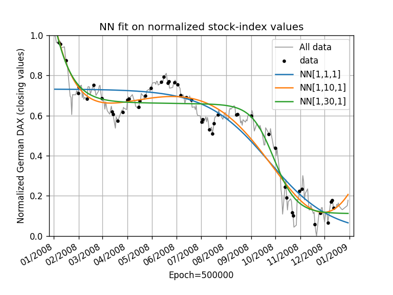
The introductory problem solved with varying neurons in the second layer
With a random initialization, the resulting NN performs disappointingly. After 0.5 million training epochs, the resulting functions are not well-fitting the data. Only a fraction of the sigmoid function can be identified in the graph. This means that many neurons are either dead or occupy the same space as other neurons. Also, a gradient-descent algorithm is not ideal as it gets trapped in local minima and runs slow in saddle points. The probability that this algorithm finds the global minima is also small. However, this problem is known, and there are various algorithms available to overcome this. These algorithms are implemented in established machine-learning tools; for examples, see TensorFlow Keras Optimizers.
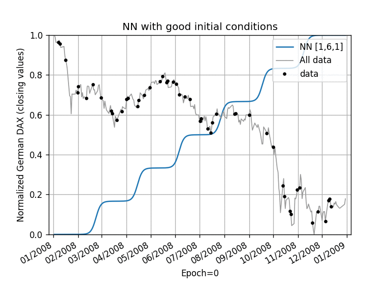
[1,6,1] NN with estimates for the initial condition (image animated)
To show the potential of NNs, in this course, the developed algorithm was used with a different set of starting conditions. The sigmoid functions were distributed equidistantly from each other and from the edges, and their heights were set to cover the y-range. These starting conditions lead to a system that can reach a relatively good approximation within hundreds of training steps.
What happens in the first 100 epochs, and why are these changes so fast?
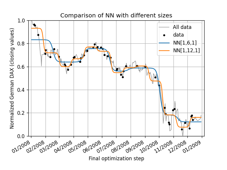
Comparison of the results of a [1,6,1] and a [1,12,1] NN
The training took place over the same amount of epochs, and the results of [1, 6, 1] and [1, 12, 1] Networks are a close approximation for the data. Deep learning is nothing more than creating a function $f(\vec{x}) = \vec{y}$ in a generalized way with (lots) of $\vec{x}$ and $\vec{y}$ datapoints. Creating NNs is neither straightforward nor easy and requires data science knowledge.
Good Questions for a Data Scientist
- Which method is used?
- How many layers are recommended to solve "this" problem?
- Which input layer is selected? Does it need to be prepared? (Fourier transformation?)
- Which output layer is selected?
- Which optimizer? And why?
Outlook
Deep Learning is just one part of machine learning. See Scikit-learn Machine Learning Map for a broad overview of problems and methods to tackle the problems.